data visualization

Load packages

library(readr)
library(here)

here() starts at C:/Users/jpatzlaff/Desktop/NCEAS/Positron Projects/Training_patzlaff

library(dplyr)

Attaching package: 'dplyr'

The following objects are masked from 'package:stats':

    filter, lag

The following objects are masked from 'package:base':

    intersect, setdiff, setequal, union

library(tidyr)
library(forcats)
library(janitor)

Attaching package: 'janitor'

The following objects are masked from 'package:stats':

    chisq.test, fisher.test

library(ggplot2)
library(plotly)

Attaching package: 'plotly'

The following object is masked from 'package:ggplot2':

    last_plot

The following object is masked from 'package:stats':

    filter

The following object is masked from 'package:graphics':

    layout

library(DT)
library(leaflet)

Load data

# read in data from tinyurl link
delta_visits_raw <- read_csv(here("data/Socioecological_monitoring_data.csv"))

Rows: 55 Columns: 13
── Column specification ────────────────────────────────────────────────────────
Delimiter: ","
chr  (4): EcoRestore_approximate_location, Reach, Time_of_Day, notes
dbl  (8): Latitude, Longitude, sm_boat, med_boat, lrg_boat, bank_angler, sci...
date (1): Date

ℹ Use `spec()` to retrieve the full column specification for this data.
ℹ Specify the column types or set `show_col_types = FALSE` to quiet this message.

Explore the data

colnames(delta_visits_raw)

 [1] "EcoRestore_approximate_location" "Reach"                          
 [3] "Latitude"                        "Longitude"                      
 [5] "Date"                            "Time_of_Day"                    
 [7] "sm_boat"                         "med_boat"                       
 [9] "lrg_boat"                        "bank_angler"                    
[11] "scientist"                       "cars"                           
[13] "notes"                          

glimpse(delta_visits_raw)

Rows: 55
Columns: 13
$ EcoRestore_approximate_location <chr> "Decker Island", "Decker Island", "Dec…
$ Reach                           <chr> "Brannan to Decker Island", "Decker Is…
$ Latitude                        <dbl> 38.10587, 38.10587, 38.08456, 38.08456…
$ Longitude                       <dbl> -121.7064, -121.7064, -121.7204, -121.…
$ Date                            <date> 2017-07-07, 2017-07-07, 2017-07-07, 2…
$ Time_of_Day                     <chr> "unknown", "unknown", "unknown", "unkn…
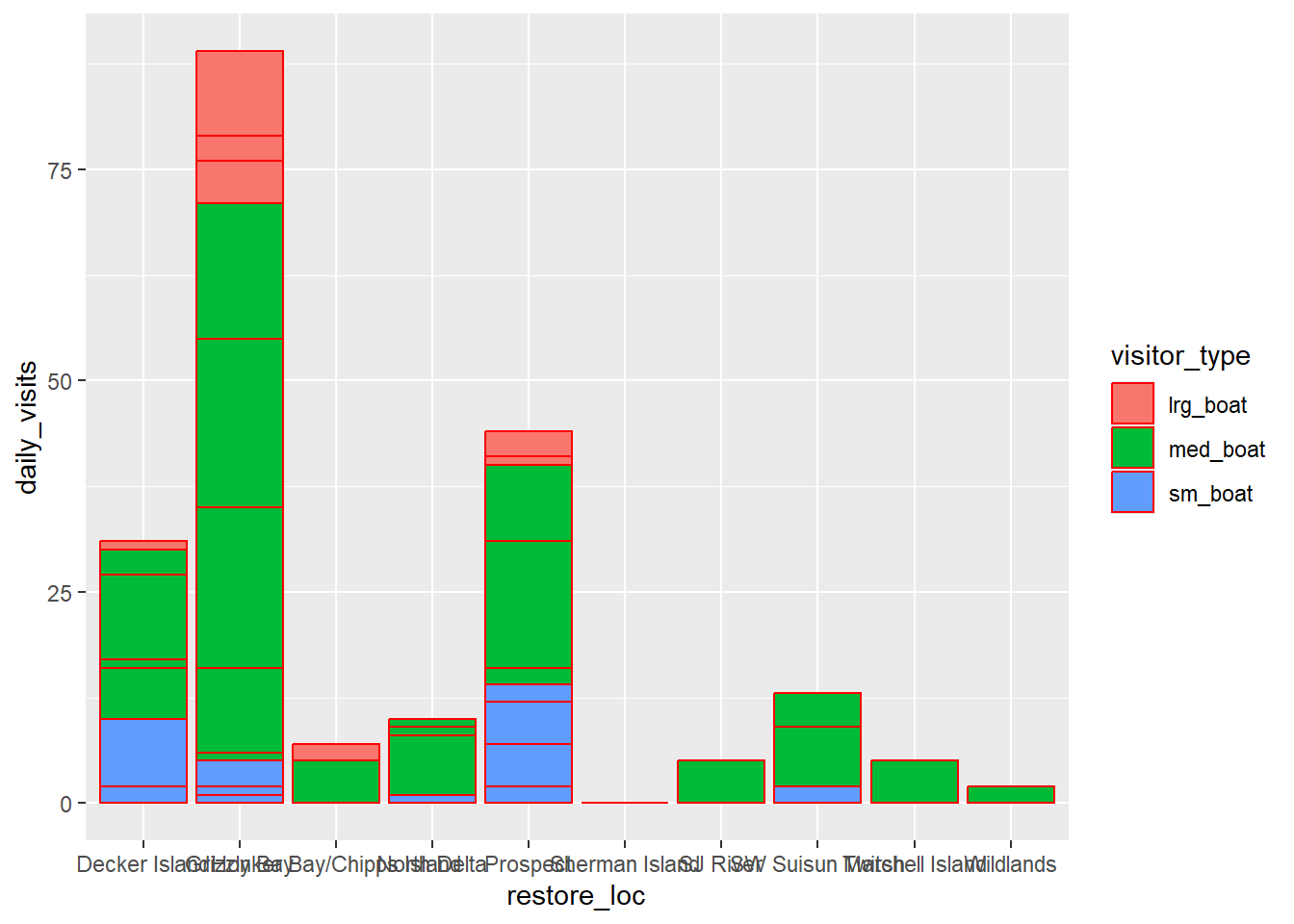
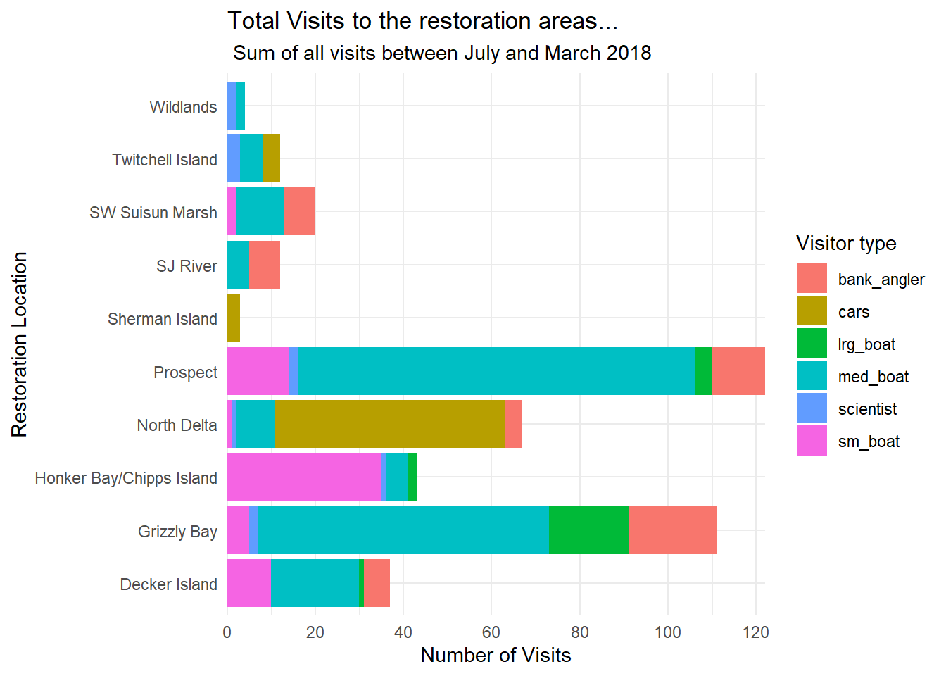
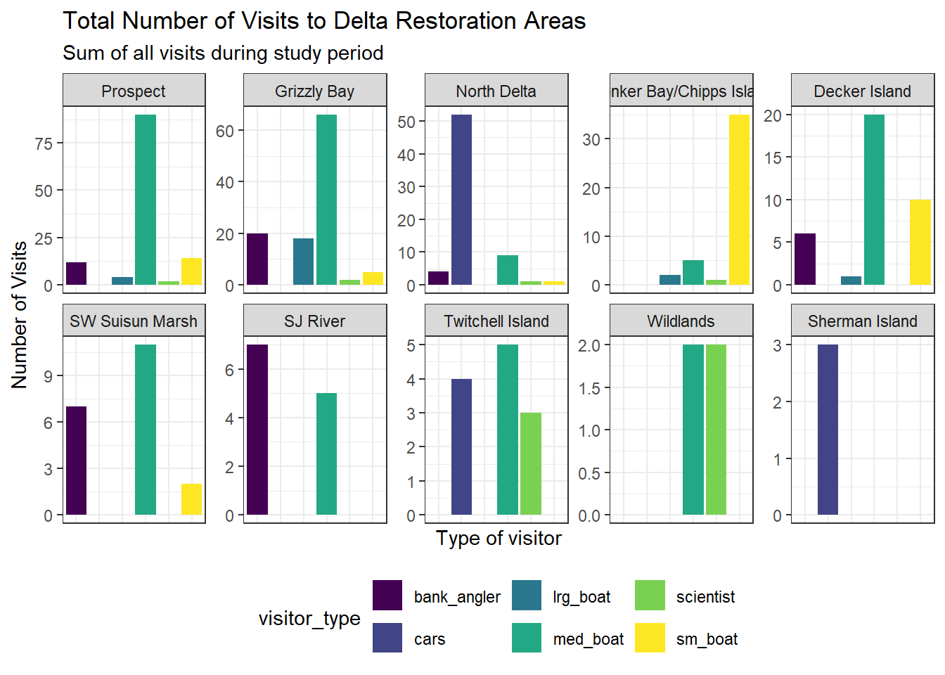
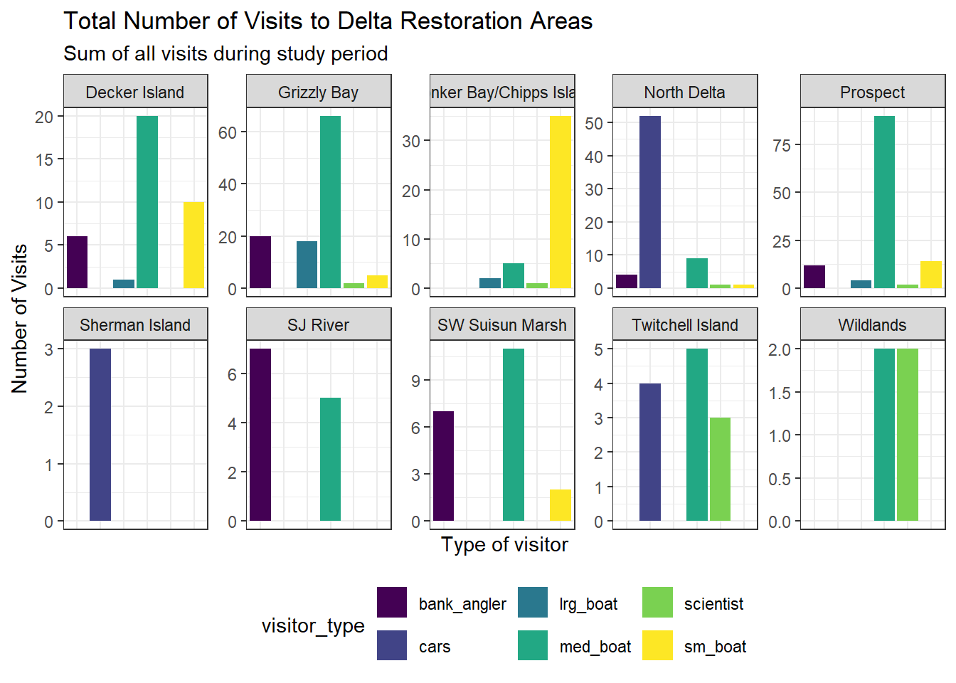
$ sm_boat                         <dbl> 0, 0, 0, 0, 2, 0, 0, 7, 1, 0, 0, 0, 0,…
$ med_boat                        <dbl> 2, 4, 0, 1, 10, 0, 0, 1, 2, 0, 1, 6, 1…
$ lrg_boat                        <dbl> 0, 0, 0, 0, 1, 0, 0, 0, 0, 0, 0, 0, 0,…
$ bank_angler                     <dbl> 1, 3, 0, 0, 0, 0, 0, 0, 2, 0, 0, 5, 0,…
$ scientist                       <dbl> 0, 0, 0, 0, 0, 0, 0, 0, 0, 0, 0, 0, 0,…
$ cars                            <dbl> 0, 0, 0, 0, 0, 0, 0, 0, 0, 0, 0, 0, 0,…
$ notes                           <chr> "no notes", "no notes", "Nobody or tra…

Clean up data

delta_visits <- delta_visits_raw %>% 
    clean_names()
delta_visits

# A tibble: 55 × 13
   eco_restore_approximate_loc…¹ reach latitude longitude date       time_of_day
   <chr>                         <chr>    <dbl>     <dbl> <date>     <chr>      
 1 Decker Island                 Bran…     38.1     -122. 2017-07-07 unknown    
 2 Decker Island                 Deck…     38.1     -122. 2017-07-07 unknown    
 3 Decker Island                 Deck…     38.1     -122. 2017-07-07 unknown    
 4 Decker Island                 Deck…     38.1     -122. 2017-09-13 unknown    
 5 Decker Island                 Bran…     38.1     -122. 2017-11-07 unknown    
 6 Decker Island                 Deck…     38.1     -122. 2017-11-07 unknown    
 7 Decker Island                 Deck…     38.1     -122. 2017-11-07 unknown    
 8 Decker Island                 Bran…     38.1     -122. 2017-12-08 morning    
 9 Decker Island                 Deck…     38.1     -122. 2017-12-08 morning    
10 Decker Island                 Deck…     38.1     -122. 2017-12-08 morning    
# ℹ 45 more rows
# ℹ abbreviated name: ¹​eco_restore_approximate_location
# ℹ 7 more variables: sm_boat <dbl>, med_boat <dbl>, lrg_boat <dbl>,
#   bank_angler <dbl>, scientist <dbl>, cars <dbl>, notes <chr>

visits_long <- delta_visits %>% 
    pivot_longer(
        col = c(sm_boat,med_boat, lrg_boat, bank_angler, scientist, cars),
        names_to = "visitor_type", 
        values_to = "quantity"
    ) %>% 
    rename(restore_loc = eco_restore_approximate_location) %>% 
    select(-notes)
glimpse(visits_long)

Rows: 330
Columns: 8
$ restore_loc  <chr> "Decker Island", "Decker Island", "Decker Island", "Decke…
$ reach        <chr> "Brannan to Decker Island", "Brannan to Decker Island", "…
$ latitude     <dbl> 38.10587, 38.10587, 38.10587, 38.10587, 38.10587, 38.1058…
$ longitude    <dbl> -121.7064, -121.7064, -121.7064, -121.7064, -121.7064, -1…
$ date         <date> 2017-07-07, 2017-07-07, 2017-07-07, 2017-07-07, 2017-07-…
$ time_of_day  <chr> "unknown", "unknown", "unknown", "unknown", "unknown", "u…
$ visitor_type <chr> "sm_boat", "med_boat", "lrg_boat", "bank_angler", "scient…
$ quantity     <dbl> 0, 2, 0, 1, 0, 0, 0, 4, 0, 3, 0, 0, 0, 0, 0, 0, 0, 0, 0, …

daily_visits_loc <- visits_long %>% 
    group_by(restore_loc, date, visitor_type) %>% 
    summarize(daily_visits = sum(quantity),.groups = "drop")
glimpse(daily_visits_loc)

Rows: 144
Columns: 4
$ restore_loc  <chr> "Decker Island", "Decker Island", "Decker Island", "Decke…
$ date         <date> 2017-07-07, 2017-07-07, 2017-07-07, 2017-07-07, 2017-07-…
$ visitor_type <chr> "bank_angler", "cars", "lrg_boat", "med_boat", "scientist…
$ daily_visits <dbl> 4, 0, 0, 6, 0, 0, 0, 0, 0, 1, 0, 0, 0, 0, 1, 10, 0, 2, 2,…

Make some plots

daily_visits_loc %>% 
    filter(daily_visits < 30,
            visitor_type %in% c("sm_boat", "med_boat", "lrg_boat")) %>% 
    ggplot(aes(x = restore_loc, y = daily_visits))+
     geom_col(color='red', 
            fill='steelblue') 

daily_visits_loc %>% 
    filter(daily_visits < 30,
            visitor_type %in% c("sm_boat", "med_boat", "lrg_boat")) %>% 
    ggplot(aes(x = restore_loc, y = daily_visits))+
     geom_col(aes(fill = visitor_type),
     color='red') 

daily_visits_loc %>% 
    ggplot(aes(y = restore_loc, x = daily_visits, fill = visitor_type))+
    geom_col()+
    labs(
        x = "Number of Visits",
        y = "Restoration Location",
        fill = "Visitor type",
        title = "Total Visits to the restoration areas...",
        subtitle = " Sum of all visits between July and March 2018"
    ) +
    scale_x_continuous(breaks = seq(0,120,20), expand = c(0,0)) + 
    theme_minimal()+
    theme(
    legend.position = "right",
    axis.ticks.y = element_blank()
    )

daily_visits_totals <- daily_visits_loc %>%
  group_by(restore_loc) %>%
  mutate(total = sum(daily_visits)) %>%
  ungroup() %>%
  mutate(restore_loc = fct_reorder(restore_loc, desc(total)))

unique(daily_visits_totals$restore_loc)

 [1] Decker Island            Grizzly Bay              Honker Bay/Chipps Island
 [4] North Delta              Prospect                 SJ River                
 [7] SW Suisun Marsh          Sherman Island           Twitchell Island        
[10] Wildlands               
10 Levels: Prospect Grizzly Bay North Delta ... Sherman Island

my_theme <- function(base_size = 14) {
    theme_minimal(base_size = base_size) +
    theme(legend.position = "bottom", 
          panel.grid.major = element_line(color = 'slateblue1'))
}

ggplot(data = daily_visits_totals,
       aes(y = restore_loc, x = daily_visits, fill = visitor_type)) +
  geom_col() +
  scale_fill_viridis_d() +
  scale_x_continuous(breaks = seq(0, 120, 20), expand = c(0, 0)) +
  labs(
    x = "Number of Visits",
    y = "Restoration Location",
    fill = "Visitor Type",
    title = "Total Visits to Delta Restoration Areas by Visitor Type",
    subtitle = "Sum of all visits during the study period"
  ) +
  my_theme()

##ggsave("figures/visit_restore_site_delta.jpg", width = 12, height = 6, units = "in")

facet_plot <- ggplot(data = daily_visits_totals,
       aes(x = visitor_type, y = daily_visits,
           fill = visitor_type)) +
    geom_col() +
    facet_wrap(~restore_loc,
               scales = "free_y",
               ncol   = 5,
               nrow   = 2) +
    scale_fill_viridis_d() +
    labs(x        = "Type of visitor",
         y        = "Number of Visits",
         title    = "Total Number of Visits to Delta Restoration Areas",
         subtitle = "Sum of all visits during study period") +
    theme_bw() +
    theme(legend.position = "bottom",
          axis.ticks.x    = element_blank(),
          axis.text.x     = element_blank())

facet_plot

facet_plot <- ggplot(data = daily_visits_loc,
       aes(x = visitor_type, y = daily_visits,
           fill = visitor_type)) +
    geom_col() +
    facet_wrap(~restore_loc,
               scales = "free_y",
               ncol   = 5,
               nrow   = 2) +
    scale_fill_viridis_d() +
    labs(x        = "Type of visitor",
         y        = "Number of Visits",
         title    = "Total Number of Visits to Delta Restoration Areas",
         subtitle = "Sum of all visits during study period") +
    theme_bw() +
    theme(legend.position = "bottom",
          axis.ticks.x    = element_blank(),
          axis.text.x     = element_blank())
facet_plot

show an interactive

delta_visits_raw <- read_csv(here("data/Socioecological_monitoring_data.csv"),
                             show_col_types = FALSE)

daily_visits_loc <- delta_visits_raw %>%
  janitor::clean_names() %>%
  tidyr::pivot_longer(
    cols      = c(sm_boat, med_boat, lrg_boat, bank_angler, scientist, cars),
    names_to  = "visitor_type",
    values_to = "quantity"
  ) %>%
  dplyr::rename(restore_loc = eco_restore_approximate_location) %>%
  dplyr::select(-notes) %>%
  dplyr::group_by(restore_loc, date, visitor_type) %>%
  dplyr::summarize(daily_visits = sum(quantity), .groups = "drop")

Interactive Table

DT::datatable(
  daily_visits_loc,
  caption  = "Daily visitor counts at Delta restoration sites",
  colnames = c("Location", "Date", "Visitor type", "Daily visits"),
  options  = list(pageLength = 10)
)

show an interactive map

Interactive Map

restoration_sites <- delta_visits_raw %>%
  janitor::clean_names() %>%
  distinct(restore_loc = eco_restore_approximate_location,
           latitude, longitude) %>%
  drop_na(latitude, longitude)

leaflet(restoration_sites) %>%
  addTiles() %>%
  addMarkers(
    lng   = ~longitude,
    lat   = ~latitude,
    popup = ~restore_loc
  )

leaflet(restoration_sites) %>%
  addTiles() %>%
  addCircleMarkers(
    lng         = ~longitude,
    lat         = ~latitude,
    popup       = ~restore_loc,
    radius      = 8,
    fillColor   = "steelblue",
    fillOpacity = 0.8,
    stroke      = FALSE
  )